ESL : support vector machine
In classification problems, linear discriminant analysis and logistic regression are methods of establishing linear decision boundaries to delineate data into classes. Separating hyperplanes could also be constructed to classify data and when they are linearly separable, we have a hard margin support vector machine. However, when classes overlap, extensions to the separating hyperplanes could be generalized to accommodate for this non-separable case (soft margin support vector machine). The goal here is to provide the best separation between two classes.
Constructing the optimal separating hyperplane reduces to a quadratic programming problem as shown in the book “The elements of statistical learning”. I will list out key important steps that led to the characterization of it as a quadratic programming problem in the case of a hard margin SVM. In the case of a hard margin SVM, there are infinitely many solutions but the best boundary is one that maximizes the distance between the data points closest to the boundary. Suppose x is a n by p vector of features and Y is a n by 1 vector of responses ($Y \in {-1, 1}$).
Define the hyperplane by : $x: f(x) = x^T\beta + \beta_0 = 0$. When $ Y_i = 1$ is mis-classified, $ f(x_i) <0$ (ie. on the other side of the plane). As such, $ y_if(x_i)>0, \forall i $ corresponds to correct classification. Then, $ \text{sign}(d_i) = \text{sign}(x_i^T\beta + \beta_0)$ refers to the classification rule. Such classifiers are known as “perceptrons”.
Properties of perceptrons:
For any two points $x_1, x_2 $ lying on the hyperplane, $ \beta^T (x_1 - x_2) = 0 $ which means that $ \beta^T$ is orthogonal to the hyperplane. Then, $ \beta*^T = \frac{\beta^T}{||\beta||}$ is a unit norm to the hyperplane. The distance of any point x to the hyperplane is given by $\beta*^{T} (x - x_0)$
Margin is defined as the distance of the hyperplane to the closest point.
Margin, M = min{$ d_iy_i$}, i = 1, … n
The objective function: $max_{\beta, \beta_0, ||\beta|| = 1} $ M, subject to $y_i (x_i^T\beta + \beta_0) \geq M, \forall i$ which simplifies to $y_i(x_i^T + \beta_0) \geq M||\beta||$. The conditions are such that all data points are at least a signed distance of M away. By arbitrarily setting up $M = 1/||\beta||$, this translates the problem into $ \text{min}_{\beta, \beta_0} \frac{1}{2} ||\beta||^2 $ s.t. $y_i(x_i^T + \beta_0) \geq 1 \forall i$. We use L2 norm because it allow us to take derivative function. This is a quadratic problem with linear inequality constraints.
Here, we can use Lagrange method (which seeks to find local minima/maxima subject to equality constraints). The Lagrangian function is $L(\beta_0, \beta, \alpha_i) = 1/2||\beta||^2 - \sum_{i=1}^{n}\alpha_i(y_i(x_i^T\beta + \beta_0) - 1) $ (each datapoint is a constraint). By taking derivative wrt $\beta$ and $\beta_0$, we have $\beta = \sum_{i=1}^n \alpha_iy_ix_i$, $0 = \sum_{i=1}^{n}\alpha_iy_i$. Substituting the representation of $\beta$ back into the above equation gives the dual
$\sum_{i=1}^{n} \alpha_i - \frac{1}{2}\sum_{i=1}^{n}\sum_{k=1}^{n}\alpha_i\alpha_ky_iy_kx_i^Tx_k $
subject to $\alpha_i \geq 0$. In addition, the problem must also satisfy $\alpha_i(y_i(x_i^T\beta + \beta_0) - 1) = 0 \forall i $ (complementary slackness of the Karush-Kuhn-Tucker conditions).
On computing the intercept term ($\beta_0$) after we have found $ \hat{\beta}$:
(This explains the computation of the intercept term ). An intuitive explanation is that, we seek an optimal $\beta_0$ such that it will be equidistant between positive and negative examples. We have the closest distance to the margin from the negative example as
$max_{i:y_i = -1} x_i^T\hat{\beta} + \beta_0 = - 1$ and the closest distance to the margin from the positive example as $\text{min}{i:y_i = 1} x_i^T\hat{\beta} + \beta_0 = 1$. Then we see that $ \beta_0 = -\frac{1}{2} [(\text{max}{i:y_i = -1} x_i^T\hat{\beta}) +(\text{min}_{i:y_i = 1} x_i^T\hat{\beta})]$.
In the case of the soft margin SVM, we include an extra term in the condition for the hyperplane (known as slack variables). This is because when classes overlap, the slack term allows some of the points to be on the wrong side of the margin.
Briefly, our condition becomes: $y_i(x_i^T\beta + \beta_0) \geq 1 - \xi_i, \forall i$ where $\xi_i \geq 0, \forall i$ is the slack variable and $\sum_{i=1}^{n}\xi_i \leq \gamma$. Doing so would require us to penalize the objective function:
$\text{min } \frac{1}{2}||\beta||^2 + \gamma\sum_{i=1}^{n}\xi_i$. Here $\gamma = 0.5$. We apply Lagrangian method as in the hard margin case. The primal function is :
\begin{align} L(\beta, \beta_0, \lambda_i, \alpha_i, \xi_i) =\\\ \frac{1}{2}||\beta||^2 + \gamma\sum_{i=1}^{n}\xi_i - \sum_{i=1}^{n}\alpha_i(y_i(x_i^T\beta + \beta_0) - 1 + \xi_i) -\sum_{i=1}^{n}\lambda_i \xi_i \end{align}
Differentiate wrt $\beta_0, \beta \text{ and } \xi_i$ and solve for $\beta$ and $\beta_0$ as before.
Code implementation:
In R, there is a package called quadprog that solves quadratic programming problem. Documentation says it solves quadratic programming problem of the form :
min ($-d^T b + 1/2 b^T D b$) with the constraints $A^T b \geq b_0$
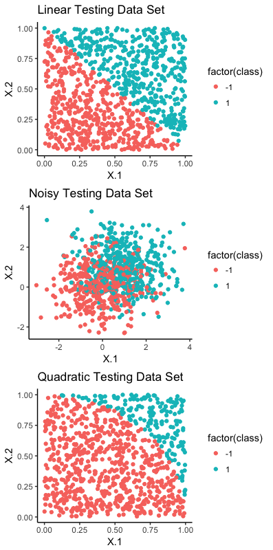
Hard- and soft-margin SVM are implemented on datasets that are linearly separable, noisy and quadratic dataset. The datasets are in .mat, however R’s R.matlab provides an interface to Matlab from R. Code and full tutorial is available on Github here. I will just illustrate the datasets and provide core results here.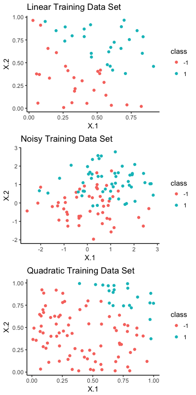
The plot above shows that both linear and quadratic data set are separable but the noisy training set has some overlap between the two classes.
We present results: accuracy and misclassification error rates on both the training and test datasets of each of the above. Note that here, it is easy to visualize the separating hyperplane on a 2D plot as we only have two features.

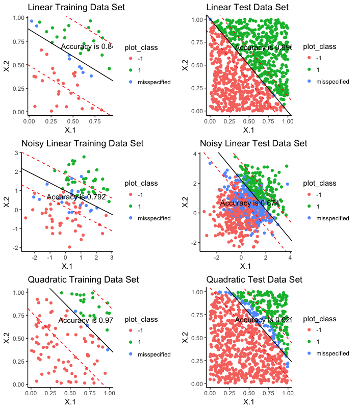
When the data is non-separable (noisy linear dataset ), SVM may not be a good choice for classification. Hard Margin SVM performs well on linearly separable dataset as we would expect, with no mis-specifications. When we use soft margin SVM, there are misspecified points Similar performance of both hard and soft margin SVM on the quadratic datasets.
This concludes my post on SVM.
References: